
The standard deviation of projectile velocity is one of the most widely cited performance metrics for long range precision shooting. Unfortunately, standard deviations are commonly misinterpreted and applied in mathematically incorrect ways. While a standard deviation is a useful statistical measure, it is important to understand what the number really means and the requisite data necessary to make valid causal inferences from a standard deviation.
Before delving into the technical details of standard deviations. It is important to consider why projectile velocity is important for long range shooting. The firing pin strikes the primer igniting the propellant charge which accelerates the projectile through the length of the barrel. When the bullet exits the barrel it is at its maximum velocity. The velocity of the projectile as it exits the barrel is referred to as the initial velocity; commonly denoted as Vo. The initial velocity (Vo) of a projectile as it exits the muzzle of the firearm is critical variable in kinematic equations of motion as it has a significant effect on the trajectory of the bullet with respect time of flight to target, drop, drift and kinetic energy.
As the bullet exits the barrel, forces such as air resistance, wind vectors (direction) and gravity begin to influence the trajectory of the bullet. Air resistance is a force acting in the direction opposite to relative motion of the bullet and acts to slow the velocity of the bullet. Atmospheric conditions such as density influence the amount of air resistance acting on a projectile. The geometry or shape of the bullet will also have an effect on the amount of air resistance encountered. The more dense the air the more resistance will be encountered by the bullet. Additionally, air resistance is a function of velocity and in laminar flow conditions the air resistance force is proportional to the velocity. Said differently, at higher velocities, there is more air resistance acting on the bullet and this force decreases as velocity decreases. With regards to wind vectors, atmospherics as well as the cross-sectional area and time of flight will influence the drift of the bullet. A larger cross sectional area results in more surface area for wind forces to act on and thus will impart more force on the projectile. It is noteworthy that cross-sectional area is a component in calculating ballistic coefficients. The time of flight is also important because the longer the bullet is in motion the more time wind forces are pushing the bullet; thus increasing drift. As a result, higher initial velocities will reduce time of flight and thus drift. Similarly, gravity also begins to act on a bullet as it leaves the barrel. Gravity is a constant force acting on the bullet while in flight. Shorter flight times mean gravity is acting on the bullet for less time and thus results in less drop. It is apparent that these forces, while not an exhaustive list of forces and factors influencing bullet flight, are highly interrelated.
Considering the forces discussed in the previous paragraph, consider how a change to the initial velocity will influence the bullet trajectory or flight path. For example, a bullet exiting the barrel faster (assuming identical geometric properties of each bullet and identical atmospheric conditions) will reach the target sooner with less drop and drift because gravity and wind vectors will act on it for shorter periods of time. If there are large variations in the initial velocity of the bullet, the trajectory will also vary. The variation in trajectory becomes more and more evident as distance increases and external forces have more time to act on the bullet. As a result, knowing and maintaining consistent initial muzzle velocity Vo is necessary for predictable, consistent and repeatable trajectories at long range.
As the variation in initial muzzle velocity increases hit probably goes down. This is because the ability to accurately apriori predict trajectory for windage and elevation adjustments becomes more difficult. It is important to note that other factors beyond just the initial velocity influence hit probability at long ranges. Some of these factors include the general precision (grouping) of a cartridge in a given rifle, bullet twist to stabilize the projectile.
Variation in a large number of factors including but not limited to propellant charge, primers, case geometry and neck tension can lead to variation or changes in initial muzzle velocity. Unfortunately, a cartridge has to be fired to determine the projectile velocity. A measure is needed to estimate how much variation can be expected from round to round when shooting.
One of the most common statistical metrics for quantifying variation in Vo muzzle velocity is a standard deviation. On the most basic level, a standard deviation is the square root of the variance and a measure of variation around a mean or average. On a very simple level, a standard deviation can be thought of as conveying information about how close to a mean/average an event is likely to be. The lower the standard deviation the closer to a mean the test results (in this case muzzle velocity) are likely to be and conversely the larger the standard deviation, the further away samples are likely to fall from the mean.
To more accurately understand what a standard deviation is doing consider how it is calculated and some of the statistical underpinnings. The most basic formula for a standard deviation is:
Population Standard Deviation Formula:
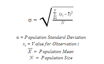
For calculation, the sample mean is calculated. The mean is subtracted from each value and squared. The resulting values are then summed together. The total sums of squares are divided by the sample size to form the population variance. The portion of the formula within the square root is the variance. The square root of the population variance variances forms the population standard deviation.
One assumption of the population variance and standard deviation is that the true mean in the population is known. Unfortunately, this is rarely the case. To review, a population is the set of all possible observations and a sample is a subset of observations from a population. Since the true population mean is generally unknown, we have to compute a mean from a sample. The difference between the sample estimated mean and the true population mean creates a bias in the estimate of the variance and standard deviation. For a normally distributed population, unless the sample mean and the population mean are equal, the squared euclidean distance or the sums of squared distance from a set of observation to a population mean will always be larger than the sum of the squared distance of a set of observations to their sample mean. As a result, the variance of a sample is biased and underestimated. Therefore, a correction factor is needed to provide a more accurate estimate.
One of the most common and nearly universally used corrections is Bessel’s correction. Bessel’s correction corrects the denominator by dividing by n-1 instead of simply n.
Bessel’s Corrected Sample Standard Deviation Formula:
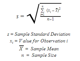
Bessel’s correction is commonly used in most ballistic calculators and statistical software packages for calculating sample standard deviations. For interpretative context, it should be noted that Bessel’s correction increases the mean squared error. Also, Bessel’s correction provides an unbiased estimate of the variance but not of the standard deviation. This is because the square root is a concave function and the concave transformation of a mean results in a value that is greater than or equal to the mean formed after such transformation. Although unbiases estimators of the standard deviation have been proposed and research has shown n-1.5 to produce asymptotically more accurate estimates, in general practice, especially considering the sample sizes often used in precision shooting, the difference between Bessel's and other corrections accounts for a relatively small proportion of the error.
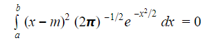
Alternatively, one can also consider the formulations with respect to a probability density function where the variance can be expressed as:
To understand a standard deviation, it is next important to understand what the number means and how it is interpreted. The central limit theorem states that if a series of samples is taken from a population, the distribution of the sample means will approach a normal distribution as n approaches infinity. This is a critical statistical and probability concept because it implies that a normal distribution can be used as an approximation for a range of problems; even when the underlying distribution itself is not necessarily normal.
A normal or Gaussian distribution has many desirable properties. The normal curve is sometimes referred to as the bell curve because of its shape. When standard deviations are calculated for muzzle velocity, the assumption is that muzzle velocity will approximate a normal distribution.

Figure 1: Normal distribution with standard deviation
To recap, a standard deviation is a measure of variation around a mean or average. The figure above illustrates a normal distribution. Numbers closer to the mean are more likely to occur than those further away from the mean. By taking a sample, in the case of precision shooting, chronographing several shots, we can calculate a standard deviation and make some inferences about how likely a given value (velocity) is to occur.
The image of the normal distribution above has a series of colored bars representing standard deviations from the mean. For 1 standard deviation above and below the mean, we expect approximately 68% of all values to fall within this range. Further, we expect 95% of observations to fall within 2 standard deviations of the mean and 99.6% to fall +/- 3 standard deviations from the mean.
Consider a cartridge with an average muzzle velocity of 2,950 ft/second and standard deviation of 10 ft/second. This means we can expect approximately 66% of shots fired to have an initial muzzle velocity between 2,940 and 2,960. Similarly, for 3 standard deviations encompasses 2,920 to 2,980. For 3 standard deviations, if 100 rounds are fired it would be reasonable to expect a maximum extreme spread of 60 ft/second.
One important factor in determining the velocity mean (average) and a standard deviation is sample size. With a small sample, the precision of the estimate is lower as it is more variable. As the sample size grows, the more confidence we have in the estimates. Consider flipping a coin 10 times. For a fair coin, there is an equal probability of it landing heads or tails. Assume we flip the coin and find 6 out of 10 times the coin lands heads, would this be enough evidence to conclude the coin is biased and more likely to land heads or might it have been random chance? Would one be willing to bet on the coin landing on heads from 10 flips? How about 100 flips in which 60 are heads and 40 are tails or 1,000 flips where 600 are heads and 400 are tails? As the sample size increase confidence in the measure increases. Similarly, note that the sample size n is a part of the denominator of the variance and standard deviation formula. Simply increasing the sample size will decrease the standard deviation due to increased precision of measure. For example, take a random series of 5 observations and calculate the standard deviation. Now copy the same 5 observations 30, 50 or 100 times and recalculate the standard deviation. One will find that despite the same observations, the increased sample size will reduce the standard deviation.
Additionally, consider the issue of sampling error. If a sample of 5 shots is taken where the true population standard deviation is 10 ft/second, while it is most likely that a majority of the velocities recorded will be within 20 fps or +/- 1sd, it is possible by chance alone to obtain a velocity value 2-3 standard deviations away. Obtaining a velocity range of 50 ft/second range or extreme spread due to one ‘outlier’ in a small sample will artificially inflate the calculation of the standard deviation. Simply seeing one somewhat aberrant velocity reading in a small sample should be evaluated in the context of what rare events should be expected for a given standard deviation. If the result appears consistently over time, it may be indicative of a larger standard deviation and expected velocity spread. Nonetheless, it is important not to unduly focus on n=1 events with small sample sizes. From the central limits theorem, typically a sample begins to approach a normal distribution with an n (sample size) of approximately 27.
An assumption underlying standard deviation calculations is that observations are independent of one another or that one measurement does not have any effect on the others. In the case of precision shooting, this is not necessarily the case. One example is barrel and receiver temperature. As rounds are fired through the barrel it heats up; sometimes quite dramatically after large shot strings. Temperature of the barrel and receiver will have effects in two ways. First, from the Ideal Gas Law Pressure * Volume = n amount of a substance * R ideal gas constant * Temperature we can see that the heating of the case and thus perhaps the propellant can cause a change in velocity. This is especially true if the ammunition is loaded with double base propellants which include nitroglycerin in the mixture. At Eagle Eye, to keep our propellants as thermally stable as possible, we only utilize single base extruded propellants without nitroglycerin. Another way temperature can cause velocity measures to be correlated is via thermal expansion of the barrel. As the barrel heats up it will begin to expand changing the contact with a projectile. As a result, it is important to consider that third variable external factors may be influencing velocity standard deviations beyond just the rifle and ammunition. Accounting for time series autocorrelations or other factors can aid in interpretation of results.
The logical question is how big of a standard deviation is acceptable or how big of a difference does a standard deviation make on results downrange. The magnitude of the difference depends on several factors such as the distance to the target and the cartridge / rifle being used.
1,000 Yard Trajectory Spread - Sea Level
| # Standard Deviations 10fps SD | 308 Win 175gr | 6.5 Creedmoor 130gr |
| 1 SD (20 fps spread) 68% of Shots | 7.2” (2,620-2,640 fps) | 4.7” (2,920-2940 fps) |
| 2 SD (40 fps spread) 95% of Shots | 14.8” (2,610-2,650 fps) | 9.3” (2,910-2,950 fps) |
| 3 SD (60 fps spread) 99.6% of Shots | 21.9” (2,600-2,660 fps) | 13.9” (2,900-2,960 fps) |
Considering distance to a target first, for a 308 Win 175gr OTM traveling at 2,600 vs 2,660 feet/second the projectile with an initial muzzle velocity of 2,600 will only drop an additional ⅓ of an inch by 200 yards compared to the projectile with a Vo of 2,660 feet/second. At short distances even large differences in velocity only produce small changes. However, at 1,000 yards the difference is 21.9”. The difference at 1,000 yards could easily be the difference between a hit/miss or dropping a point in competition. However, for a 6.5 Creedmoor 130gr with an initial velocity of 2,900 feet/second versus one traveling at 2,960 feet/second the difference at 200 yards will only be 0.2” and at 1,000 yards the difference will be 13.9” (calculations assuming sea level elevation, 30inHg barometric pressure and 59 deg f). At short distances the difference in the two cartridges is minimal. However, since the 6.5 creedmoor projectile is traveling faster, the force of gravity will be acting on it for a shorter period of time as it travels to the target. As a result, despite the same extreme spread or velocity standard deviation, the magnitude of the initial velocity effect is less.
Similarly, for a standard deviation of 10, a +/- one standard deviation would equate to a velocity range of 20 feet/second and 68% of the shots fired would be expected to fall within this range. For the same 308 Win 175gr cartridge, a V0 of 2,620 feet/second vs a V0 of 2,640 feet/second would have only 0.1” difference at 200 yards in trajectory drop and 7.2” at 1,000 yards. The 1,000 yard trajectory difference is approximately ⅓ of the 3 standard deviation estimate. Similarly, as can be seen in the above table, a one standard deviation spread for a 6.5 Creedmoor 130gr loading equates to approximately 4.7” spread; considerably less than a 3 sd spread.
If we consider a standard deviation of 5 feet/second we would expect 99.6% of the velocities to be less than the 2sd spreads in the above table for a 10 fps sd. This is because 5*6 (3sd+ and 3sd- the mean) is 30 feet/second whereas a 2 sd spread at an sd of 10 is 40 feet/second.
The primary question is how much does standard deviation matter and what is a good standard deviation? It depends on the distance, caliber, target and tolerance for error. As we saw above, for a flatter shooting cartridge there is less of a difference. The 6.5 Creedmoor’s higher velocity compared to a 308 Win and its flatter trajectory is less perturbed by variations in muzzle velocity. At short distances, such as as few hundred yards, the difference in muzzle velocity is on the order of tenths of an inch. For hunting or plinking a few tenths of an inch may be less critical than for benchrest competition.
When considering the actual standard deviation itself, one way to put the change into context is regarding hit probability. Assuming all other factors such as wind, shooter error, dispersion etc are held constant, if we just consider the standard deviation at long range shooting we can get a feel for how much of a difference a change in sd means to a shooter. For example, a ½ IPSC target is 16” tall. For a 6.5 Creedmoor we would expect nearly all of the projectiles to have a spread of less than 16” for both a standard deviation of 5 and 10 feet/second. In one sense, the change is negligible. However, it can also be argued that more consistency adds margin for error in other factors and will reduce error when considering mean dispersion from shooter group size. With regards to 308, we would expect approximately 96-97% of shots to be within an ½ IPSC at a 10 feet/second sd and nearly all at an sd of 5. In this regard, the difference equates to only a few percent increase in hit probability. For F-Class shooters where a 10” change results in the dropping of an X or a point, lowering the standard deviation may be more critical.
Velocity standard deviations are a useful metric for quantifying expected variation in muzzle velocities and the resulting downrange dispersion. When interpreting a standard deviation, it is important to consider the sample size used to calculate the sd and to place the extreme spread in the context of the sample size. With small samples, the precision of the estimate can biased and one observation can dramatically skew a standard deviation calculation in small samples. When considering the downrange implications of a standard deviation, it is important to consider the ballistic profile of the rifle and cartridge combination in a given atmospheric condition. For some calibers at a given distance, the effect of a larger/smaller standard deviation may equate to different downrange performance characteristics. While there is no downside to a lower velocity standard deviation, it is important to keep in context the difference, and sometimes incremental difference it corresponds to downrange.